Tutorials Home Reading and Checking Your Data Reading CSV Data
Reading CSV Data
How to read in a single CSV, how to use RStudio's data import tool, how to read in and combine multiple CSVs.
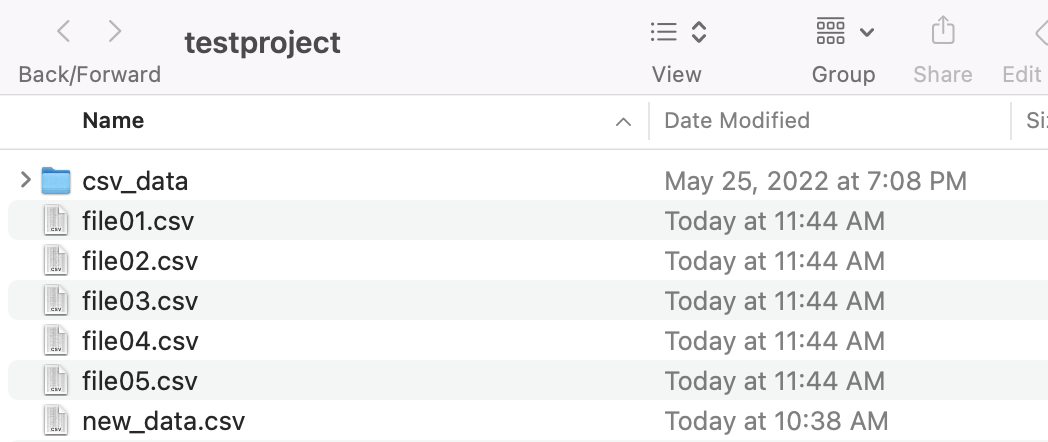
You should have already downloaded the CSV files by clicking the button above. You will have a folder with five files that will be used for this tutorial. The data is fake, I generated it for this tutorial using a few R packages and base functions. This tutorial will discuss several ways to read and write CSV data.
Reading in a Single CSV with Code
The first file we’re going to use is called reading_data.csv. There are some differences between this and tidyverse read_csv which I will explain. Keep in mind that you will need to change the file path to your local file path (wherever you keep your data) for the code in this tutorial to work.
Base R read.csv
First, let’s try the base R “read.csv” function. After reading in the data, you can use str() to check out its structure. Here we can see that the data has been read in as a data.frame, and then examine the column types.
#replace everything except "reading_data.csv" with your file location
df <- read.csv("csv_data/reading_data.csv")

str(df)
## 'data.frame':	1000 obs. of  12 variables:
##  $ id          : int  1 2 3 4 5 6 7 8 9 10 ...
##  $ first_name  : chr  "Marcus" "Daniel" "Darian" "Sultana" ...
##  $ last_name   : chr  "Goecke" "Baclayon" "Stanfield" "al-Farooq" ...
##  $ gender      : chr  "Male" "Male" "Male" "Female" ...
##  $ race        : chr  "White" "Asian/Pacific Islander" "Black/African American" "Middle Eastern" ...
##  $ age         : num  44.2 33.6 29.5 47.5 42 ...
##  $ dob         : chr  "1978-03-02" "1988-10-13" "1992-11-18" "1974-11-09" ...
##  $ company     : chr  "Daugherty Inc" "Rempel-Rempel" "Kuphal LLC" "Miller LLC" ...
##  $ job         : chr  "Data scientist" "Nurse, mental health" "Building services engineer" "Leisure centre manager" ...
##  $ fav.IceCream: chr  "Oreo" "Chocolate" "Vanilla" "Chocolate" ...
##  $ review_date : chr  "2020-09-17T12:00:00Z" "2019-12-06T12:00:00Z" "2019-12-31T12:00:00Z" "2020-08-02T12:00:00Z" ...
##  $ score       : int  5 3 4 4 5 3 3 4 5 5 ...
Tidyverse read_csv
When you use tidyverse read_csv, you’ll get this message telling you a bit more about the file you’re reading in.
tbl_df <- read_csv("csv_data/reading_data.csv")
Now this time the data was read in as a tibble instead of a data.frame. Check out this short vignette or type vignette(“tibble”) in your console for more info on the differences between tibbles and dataframes. You can see that all of the numeric columns were read in as numeric with read_csv, but with read.csv some are integers and some are numeric. This might not matter too much to you. The other main difference is that read.csv read in the dates as character strings, but read_csv reads them in as dates.
str(tbl_df)
## spec_tbl_df [1,000 × 12] (S3: spec_tbl_df/tbl_df/tbl/data.frame)
##  $ id          : num [1:1000] 1 2 3 4 5 6 7 8 9 10 ...
##  $ first_name  : chr [1:1000] "Marcus" "Daniel" "Darian" "Sultana" ...
##  $ last_name   : chr [1:1000] "Goecke" "Baclayon" "Stanfield" "al-Farooq" ...
##  $ gender      : chr [1:1000] "Male" "Male" "Male" "Female" ...
##  $ race        : chr [1:1000] "White" "Asian/Pacific Islander" "Black/African American" "Middle Eastern" ...
##  $ age         : num [1:1000] 44.2 33.6 29.5 47.5 42 ...
##  $ dob         : Date[1:1000], format: "1978-03-02" "1988-10-13" ...
##  $ company     : chr [1:1000] "Daugherty Inc" "Rempel-Rempel" "Kuphal LLC" "Miller LLC" ...
##  $ job         : chr [1:1000] "Data scientist" "Nurse, mental health" "Building services engineer" "Leisure centre manager" ...
##  $ fav IceCream: chr [1:1000] "Oreo" "Chocolate" "Vanilla" "Chocolate" ...
##  $ review_date : POSIXct[1:1000], format: "2020-09-17 12:00:00" "2019-12-06 12:00:00" ...
##  $ score       : num [1:1000] 5 3 4 4 5 3 3 4 5 5 ...
##  - attr(*, "spec")=
##   .. cols(
##   ..   id = col_double(),
##   ..   first_name = col_character(),
##   ..   last_name = col_character(),
##   ..   gender = col_character(),
##   ..   race = col_character(),
##   ..   age = col_double(),
##   ..   dob = col_date(format = ""),
##   ..   company = col_character(),
##   ..   job = col_character(),
##   ..   `fav IceCream` = col_character(),
##   ..   review_date = col_datetime(format = ""),
##   ..   score = col_double()
##   .. )
##  - attr(*, "problems")=<externalptr>
I pretty much always use read_csv as the default. If you have a large dataset, reader::read_csv should be faster than base read.csv. Now, there are a few more things you can do to customize how your file is read in, but I will use the RStudio file import tool to illustrate those points.
Using the RStudio File Import Tool
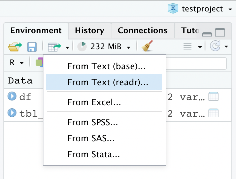
If you’re very new to R, or if you have very messy data, you might want to use one of RStudio’s built-in features. Go to your environment pane and click the data table icon with the green arrow. You’ll be able to select from a couple of different options—if you choose “From Text (base)”, you’ll be using the read.csv function. I’m going to use “From Text (readr)” which is our read_csv.
I’ve highlighted a couple of spots on the screenshot. First of all, you can either paste a link into the File/URL spot, or you can use the file browser to find the file you want to read in. If you click on one of the column headers you’ll get a dropdown menu that allows you to change the data type. Those specifications, along with your chosen delimiter, name, and any other changes you make to the file will show up in the file explorer before you read in your data.
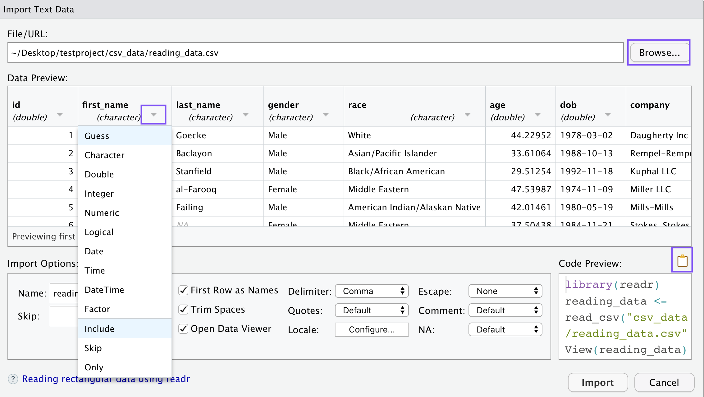
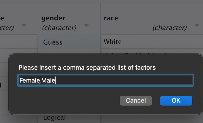
So I’ll make a few changes here— I renamed the file “new_data”, changed the ID column from double to character, and change the gender to factor. To do that, you have to provide a list of the factor’s levels.
Then copy the code in the far right-hand corner, and click “import”. You’ll usually want to do this so that you can reuse the same code to read in your data when you use the file again. Now you can see below that my code captures all of the information I changed visually in the file explorer. One thing to note, don’t worry about changing the date columns to date format. They will still be read in as dates automatically even though it looks like they’ll be read in as numeric.
new_data <- read_csv("csv_data/reading_data.csv",
    col_types = cols(id = col_character(),
        gender = col_factor(levels = c("Female",
            "Male"))))
Cleaning Column Names
Usually as soon as I read in data I use janitor::clean_names() to clean/standardize the column names. By default, this function will force all the column names to lowercase with underscores in between words, numbers, etc. I purposefully gave the “fav IceCream” column a messy name to illustrate what this function does. If you have a messy column name you can still access it by wrapping it with ``, but it is very inconvenient to do this all the time.
count(new_data, `fav IceCream`)
## # A tibble: 10 × 2
##    `fav IceCream`          n
##    <chr>               <int>
##  1 Banana                 50
##  2 Chocolate             267
##  3 Coffee                 33
##  4 Cookie Dough           75
##  5 Matcha                  9
##  6 Mint chocolate chip    46
##  7 Oreo                   91
##  8 Pistachio              20
##  9 Strawberry            117
## 10 Vanilla               292
After using clean names, you can see that it not only takes away the empty space, it also separates the words “ice” and “cream”.
new_data %>%
  clean_names() %>%
  count(fav_ice_cream)
## # A tibble: 10 × 2
##    fav_ice_cream           n
##    <chr>               <int>
##  1 Banana                 50
##  2 Chocolate             267
##  3 Coffee                 33
##  4 Cookie Dough           75
##  5 Matcha                  9
##  6 Mint chocolate chip    46
##  7 Oreo                   91
##  8 Pistachio              20
##  9 Strawberry            117
## 10 Vanilla               292
You can also customize how the column names are changed. For example, you can use snake case, set all the names to uppercase, etc.
Renaming just one column is easy to do with dplyr. You can rename multiple columns in the same rename() if you separate each set with a comma.
new_data <- new_data %>%
  rename(fav_ice_cream = `fav IceCream`)
Another thing you can do is use set_names(), which can be useful if you have a crosstab you want to print out (just as an example). If I use count(), it will give me a new column named “n”.
new_data %>%
  count(gender)
## # A tibble: 3 × 2
##   gender     n
##   <fct>  <int>
## 1 Female   475
## 2 Male     480
## 3 <NA>      45
I could use set_names() to rename these two columns. It’s a bit shorter than using rename().
new_data %>%
  count(gender) %>%
  set_names(c("Gender", "Count"))
## # A tibble: 3 × 2
##   Gender Count
##   <fct>  <int>
## 1 Female   475
## 2 Male     480
## 3 <NA>      45
You can also rename several columns at once. Use rename_with(), the first argument is the data, the second is the function you want to use to change the column name, and the third argument is the columns you want to change. If you wanted to rename all the columns, you don’t have to select anything, it will automatically perform the function on all columns like so:
rename_with(new_data,
            str_to_upper) %>%
  head()
## # A tibble: 6 × 12
##   ID    FIRST_NAME LAST_NAME GENDER RACE            AGE DOB        COMPANY JOB
##   <chr> <chr>      <chr>     <fct>  <chr>         <dbl> <date>     <chr>   <chr>
## 1 1     Marcus     Goecke    Male   White          44.2 1978-03-02 Daughe… Data…
## 2 2     Daniel     Baclayon  Male   Asian/Pacifi…  33.6 1988-10-13 Rempel… Nurs…
## 3 3     Darian     Stanfield Male   Black/Africa…  29.5 1992-11-18 Kuphal… Buil…
## 4 4     Sultana    al-Farooq Female Middle Easte…  47.5 1974-11-09 Miller… Leis…
## 5 5     Benjamin   Failing   Male   American Ind…  42.0 1980-05-19 Mills-… Surv…
## 6 6     Shafee'a   <NA>      Female Middle Easte…  37.5 1984-11-21 Stokes… Airl…
## # … with 3 more variables: FAV_ICE_CREAM <chr>, REVIEW_DATE <dttm>, SCORE <dbl>
That changed all the columns to uppercase. We could get more specific, and just select certain columns. I could also use a different function, for example add a prefix or suffix to each of my selected columns. I’m using paste0 which doesn’t add any spaces between the things you’re pasting (it’s just shorter), which is why I’ve added the underscore before “_new”. I’m also using the tidyselect function “ends_with” to select both of the “name” columns in my dataset. I can also use other tidyselect functions for this, like starts_with(), contains(), select by column names, by column position, etc.
rename_with(new_data,
            ~paste0(., "_new"),
            ends_with("name")
            ) %>%
  head()
## # A tibble: 6 × 12
##   id    first_name_new last_name_new gender race    age dob        company job
##   <chr> <chr>          <chr>         <fct>  <chr> <dbl> <date>     <chr>   <chr>
## 1 1     Marcus         Goecke        Male   White  44.2 1978-03-02 Daughe… Data…
## 2 2     Daniel         Baclayon      Male   Asia…  33.6 1988-10-13 Rempel… Nurs…
## 3 3     Darian         Stanfield     Male   Blac…  29.5 1992-11-18 Kuphal… Buil…
## 4 4     Sultana        al-Farooq     Female Midd…  47.5 1974-11-09 Miller… Leis…
## 5 5     Benjamin       Failing       Male   Amer…  42.0 1980-05-19 Mills-… Surv…
## 6 6     Shafee'a       <NA>          Female Midd…  37.5 1984-11-21 Stokes… Airl…
## # … with 3 more variables: fav_ice_cream <chr>, review_date <dttm>, score <dbl>
Reading Multiple CSV Files
This is all fine if I need to read in one or two files. But what if I had 100 files I wanted to read in and combine? It would be pretty inconvenient to write out all that code, or even copy and paste that many times. Thankfuly there’s an easier way!
First, get a list of the files in your folder directory. You’ll want to paste in your full file path up to the folder that holds your data. Or if you’re using a project and your data is in your project working directory, you can do what I did below. The dot represents the working directory, and I had to specify my folder “csv_data” because it’s a subfolder within my working directory.
files <- list.files(path = "./csv_data", pattern = "csv*", full.names = T)

files
## [1] "./csv_data/file01.csv"       "./csv_data/file02.csv"
## [3] "./csv_data/file03.csv"       "./csv_data/file04.csv"
## [5] "./csv_data/file05.csv"       "./csv_data/reading_data.csv"
I want to read in file01-file05, but not reading_data.csv. In this case, I could just truncate the list of files so I only take the first five items.
files[1:5]
## [1] "./csv_data/file01.csv" "./csv_data/file02.csv" "./csv_data/file03.csv"
## [4] "./csv_data/file04.csv" "./csv_data/file05.csv"
But what if I have a whole big list of files with messy names? I might not want to go through them and figure out every single file position I want to keep or exclude. If that were the case, I could do something like this instead:
keep(files, ~str_detect(., "file0"))
## [1] "./csv_data/file01.csv" "./csv_data/file02.csv" "./csv_data/file03.csv"
## [4] "./csv_data/file04.csv" "./csv_data/file05.csv"
The “keep” function is from the purrr package which is loaded automatically with the tidyverse. You can also go the opposite way and use discard if it’s easier—like this:
files <- discard(files, ~str_detect(., "read"))

files
## [1] "./csv_data/file01.csv" "./csv_data/file02.csv" "./csv_data/file03.csv"
## [4] "./csv_data/file04.csv" "./csv_data/file05.csv"
Okay, now that I’ve cut the list down to only the files I want to read in, I can do a couple of different things. One way to do it would be using lapply and reading into a list of tibbles. I need to name the items in the list, that will be important for the next step. Since I only have five files I could just do it manually. But again, I might have a bunch of files and I don’t want to write out a long list of dataframe names. So I’ll use the “files” list that I already have to create those names. I’m just using regular expressions and the word() function from the stringr package to accomplish this.
Now say for example I have five different datasets with different information, and I just want to read them all in and load them into my R session so I can use them as needed. After I create the list of tibbles, I can just use list2env to unpack the list into my global environment. The list must be a named list for this to work, which is why I said that would be important in the previous step.
list2env(df_list, .GlobalEnv)
## <environment: R_GlobalEnv>
Now the files are all in the global environment.
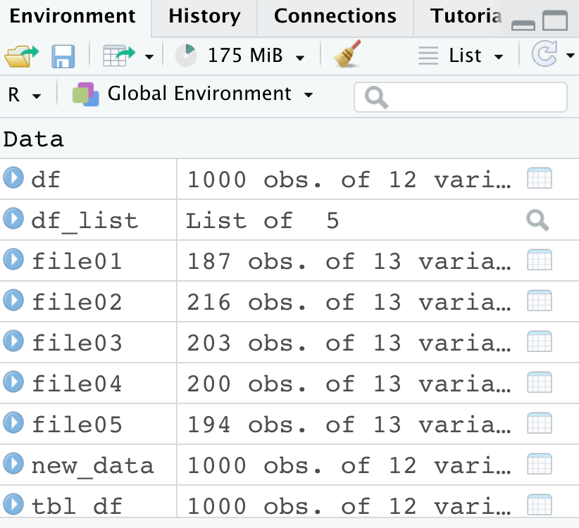
Combining Multiple CSVs
In the previous example, I demonstrated what to do if you have lots of different files you want to read at once. These are files I created for this tutorial and they are actually just subsets of the larger csv file with 1000 rows. You might have a situation where you have several CSVs that have the same data/structure, but from different time periods for example. In that case, you can also read in the files and combine them in one step.
Combining Multiple CSVs with bind_rows
So let’s take the list of dataframes already created in the last step. One thing you could do is simply use the bind_rows() function which will stack the dataframes on top of each other. The result is a tibble with 1,000 rows and 13 columns, same as our original CSV from the first step in the tutorial.
test <- bind_rows(df_list)

glimpse(test)
## Rows: 1,000
## Columns: 13
## $ id             <dbl> 5, 6, 8, 15, 23, 52, 64, 66, 72, 74, 80, 82, 93, 94, 98…
## $ first_name     <chr> "Benjamin", "Shafee'a", "Nawaar", "Megan", "Michael", "…
## $ last_name      <chr> "Failing", NA, "el-Iman", "Yazzie", "Foster", "Nunley",…
## $ gender         <chr> "Male", "Female", "Female", "Female", "Male", "Male", "…
## $ race           <chr> "American Indian/Alaskan Native", "Middle Eastern", "Mi…
## $ age            <dbl> 42.01461, 37.50438, 38.60476, 37.65556, 31.17282, 44.76…
## $ dob            <date> 1980-05-19, 1984-11-21, 1983-10-16, 1984-09-27, 1991-0…
## $ company        <chr> "Mills-Mills", "Stokes, Stokes and Stokes", "Thompson-T…
## $ job            <chr> "Surveyor, building", "Airline pilot", "Government soci…
## $ `fav IceCream` <chr> "Vanilla", "Vanilla", "Vanilla", "Vanilla", "Chocolate"…
## $ review_date    <dttm> 2017-03-24 12:00:00, 2017-10-20 12:00:00, 2017-12-27 1…
## $ score          <dbl> 5, 3, 4, 5, 2, 4, 4, 5, 5, 4, 3, 5, 5, 5, 2, 4, 4, 5, 4…
## $ review_year    <dbl> 2017, 2017, 2017, 2017, 2017, 2017, 2017, 2017, 2017, 2…
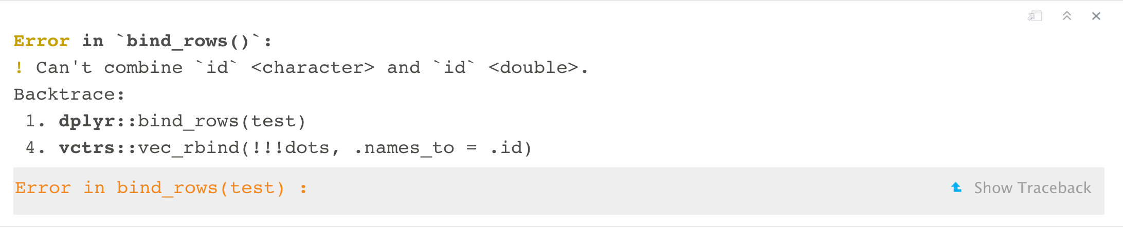
Note that this will only work if your data is in fact the same— meaning all column types with the same names should be the same. Watch what happens if we change the ID column in just the first dataframe of df_list to a character instead of numeric. They won’t combine because they’re different types so we get an error.
Also note that the structure doesn’t necessarily have to be the same. If we add a column to the first tibble in df_list, it will still work. You will get the same result only now we have 14 columns instead of 13. The test column we named “new_col” will only be filled out for the rows that were in file01, the rest of the rows for that column will be NA.
test <- df_list

test$file01$new_col <- "test column data"

bind_rows(test) %>% dim()
## [1] 1000 14
Combining Columns using coalesce()
That behavior could actually be useful to us. Let’s say we have four files where the column names are the same, but in the most recent file, the ID column was named something else. I’m going to manually change the column name to illustrate the point. Now we can see again there are 14 columns, and I know two of these represent the same data, they just have different names. The “id” column has 194 missing values, which are stored in “ID_col”.
test <- df_list

test$file05 <- test$file05 %>% rename("ID_col" = id)

test <- bind_rows(test)

summary(test$id)
##    Min. 1st Qu.  Median    Mean 3rd Qu.    Max.    NA's
##     1.0   252.2   507.5   504.7   760.5  1000.0     194
Now we can use this handy dpylr function coalesce(), which SQL users might find familiar. What this does, is use the two columns to fill in each other’s missing values. If a row in “id” is NA, but “ID_col” is not NA, it will be filled in with the value in ID_col. One important thing to note with this is that whichever column you put first inside the coalesce() function (in this case it’s ID_col) will be the default for filling in missing values. So if both id and ID_col are non-NA, the data in ID_col will stay, and it will ignore whatever data is in “id”. In this case, it doesn’t matter because I know that the NAs in both columns are mutually exclusive. But there are other times where I’ve used this function and it was important to prioritize one column over another. In any case, now we can see after using coalesce, there are no longer NAs in our ID column.
test <- test %>%
  mutate(id = coalesce(ID_col, id))

summary(test$id)
##    Min. 1st Qu.  Median    Mean 3rd Qu.    Max.
##     1.0   250.8   500.5   500.5   750.2  1000.0
Combine Multiple CSVs with purrr
There is another way to combine the dataframes from our list. If I wanted to, I could use map() first to perform other data cleaning operations, standardize the datasets prior to combining them, and all that good stuff. For example, here I’m using clean_names() on all the datasets, and changing the the age column to character format instead of numeric. Then I want to use map_df() which will combine all of our dataframes. We have to use a function, which is going to be bind_rows just like before (it could also be bind_cols, or something else).
df_list %>%
  map(. %>%
        clean_names() %>%
        mutate(age = as.character(age))) %>%
  map_df(.,
         bind_rows,
         .id = "source") %>%
  head()
## # A tibble: 6 × 14
##   source    id first_name last_name gender race   age   dob        company job
##   <chr>  <dbl> <chr>      <chr>     <chr>  <chr>  <chr> <date>     <chr>   <chr>
## 1 file01     5 Benjamin   Failing   Male   Ameri… 42.0… 1980-05-19 Mills-… Surv…
## 2 file01     6 Shafee'a   <NA>      Female Middl… 37.5… 1984-11-21 Stokes… Airl…
## 3 file01     8 Nawaar     el-Iman   Female Middl… 38.6… 1983-10-16 Thomps… Gove…
## 4 file01    15 Megan      Yazzie    Female Ameri… 37.6… 1984-09-27 Rohan … Opht…
## 5 file01    23 Michael    Foster    Male   Asian… 31.1… 1991-03-23 Thomps… Scie…
## 6 file01    52 Kristopher Nunley    Male   Ameri… 44.7… 1977-08-17 Kling,… Esta…
## # … with 4 more variables: fav_ice_cream <chr>, review_date <dttm>,
## #   score <dbl>, review_year <dbl>
The reason I wanted to show this function is because it can be very useful to label each of the dataframes while they’re combined. In the code above, the “.id =” is not referring to the column name “id” in our dataset. It’s telling the map_df() function that I want to create an id column to let me know what dataset each row is from once they are all combined. I chose to name this column “source”, but you could name it whatever you want.
Writing CSV Data
Writing one CSV is quite similar to reading it in. Using the write_csv() function you simply put the name of your dataframe first, and the file path second. Note that I’m still in my “testproject” R project, so this will be saved in my working directory because I didn’t specify a full file path.
write_csv(new_data, "new_data.csv")
Writing Multiple CSVs with mapply()
What if I wanted to write out several CSVs at one time? For example, when I unpacked the df_list into my global environment - maybe I made changes to all of those datasets separately, but now I want to save the revised files out to a folder. Here I’ve created a named list in one step, rather than creating the list and then assigning names to it. Both of these methods have the same result, so you can do whatever you find easier.
new_df_list <- list("file01" = file01,
                    "file02" = file02,
                    "file03" = file03,
                    "file04" = file04,
                    "file05" = file05)
Now I can use mapply on the list. This code is basically telling R to use write_csv on each item in new_df_list, and the file name should be the name of the list item with “.csv” at the end. If you wanted to save this in a different folder, you could specify that folder before the names(new_df_list), separated by a comma. like this:
paste0(“different_folder/”, names(new_df_list), “.csv”)
mapply(write_csv,
       new_df_list,
       paste0(names(new_df_list), ".csv"))
##              file01        file02        file03        file04
## id           numeric,187   numeric,216   numeric,203   numeric,200
## first_name   character,187 character,216 character,203 character,200
## last_name    character,187 character,216 character,203 character,200
## gender       character,187 character,216 character,203 character,200
## race         character,187 character,216 character,203 character,200
## age          numeric,187   numeric,216   numeric,203   numeric,200
## dob          Date,187      Date,216      Date,203      Date,200
## company      character,187 character,216 character,203 character,200
## job          character,187 character,216 character,203 character,200
## fav IceCream character,187 character,216 character,203 character,200
## review_date  POSIXct,187   POSIXct,216   POSIXct,203   POSIXct,200
## score        numeric,187   numeric,216   numeric,203   numeric,200
## review_year  numeric,187   numeric,216   numeric,203   numeric,200
##              file05
## id           numeric,194
## first_name   character,194
## last_name    character,194
## gender       character,194
## race         character,194
## age          numeric,194
## dob          Date,194
## company      character,194
## job          character,194
## fav IceCream character,194
## review_date  POSIXct,194
## score        numeric,194
## review_year  numeric,194
That is a little bit inconvenient because it prints out all this output, which I might not want. I could change the above code chunk to “r include=FALSE” which would only run the code and not show the output.
Writing Multiple CSVs with purrr
I could also use purrr::walk. This works just like map, except it doesn’t print out any output. So you could replace “walk2” with “map2” in the code below, and it would save the CSVs to your working directory but would also print out all the dataframes in your console, or inline if you’re using an RMarkdown document.
walk2(df_list,
      paste0(names(df_list), ".csv"),
      ~write_csv(.x, .y))
The syntax with walk is a bit different than mapply. We have to give it the list object first, then specify the file paths it should write to. Finally, specify that it should use write_csv to save out the files. The .x corresponds to the df_list, and .y corresponds to the file paths. This is because we’re using walk2, which takes two arguments and evaluates them in parallel. Map and walk take one argument, map2 and walk2 are of course two arguments, and pmap or pwalk will take multiple arguments.
Now you can see that files01-05 have been saved in my project working directory, along with the new_data.csv file that we saved out at the beginning of the tutorial.