Getting Started

Download R and RStudio

Download the latest release of R for your system:

• R for Windows
• R for MacOS

Install it to your system (the defaults should be fine).

After downloading R, you can download RStudio here. Scroll down and pick the “Rstudio Desktop” free version. Install and open RStudio. It should find your system’s R installation and connect to it automatically. You can check it using “getRversion()” and it should show whatever version you installed in the console at the bottom. This is also where your code and output will show up.

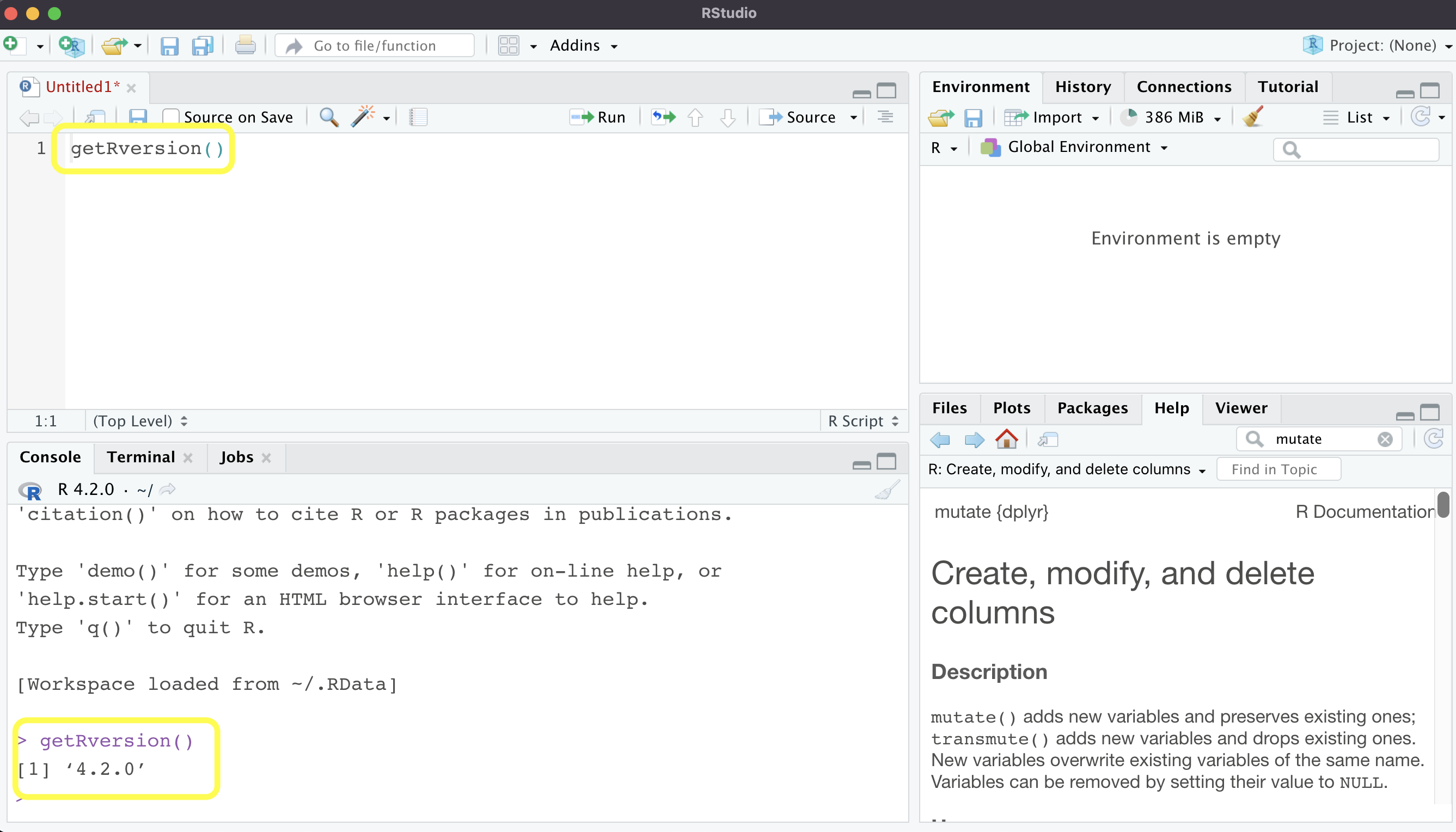
Now for the layout, you should see something similar to the screenshot above. Rstudio doesn’t automatically open a code file for you, but you can just go to File -> New File -> R Script to open one up. This is the “Untitled” document you see on the top left pane. The top right pane shows the global environment (don’t worry about the other tabs for now). This is where your data files will show up when you load them into R.

On the bottom right are several tabs that you’ll use quite often. The Files tab shows your file directory. Under “Packages” you can see which packages you have installed, and there are also buttons for installing and updating packages. Under “Help” you can search for functions and see their explanations and examples—the screenshot shows the help page for dplyr::mutate. Plots and Viewer are pretty self explanatory.

Installing Packages

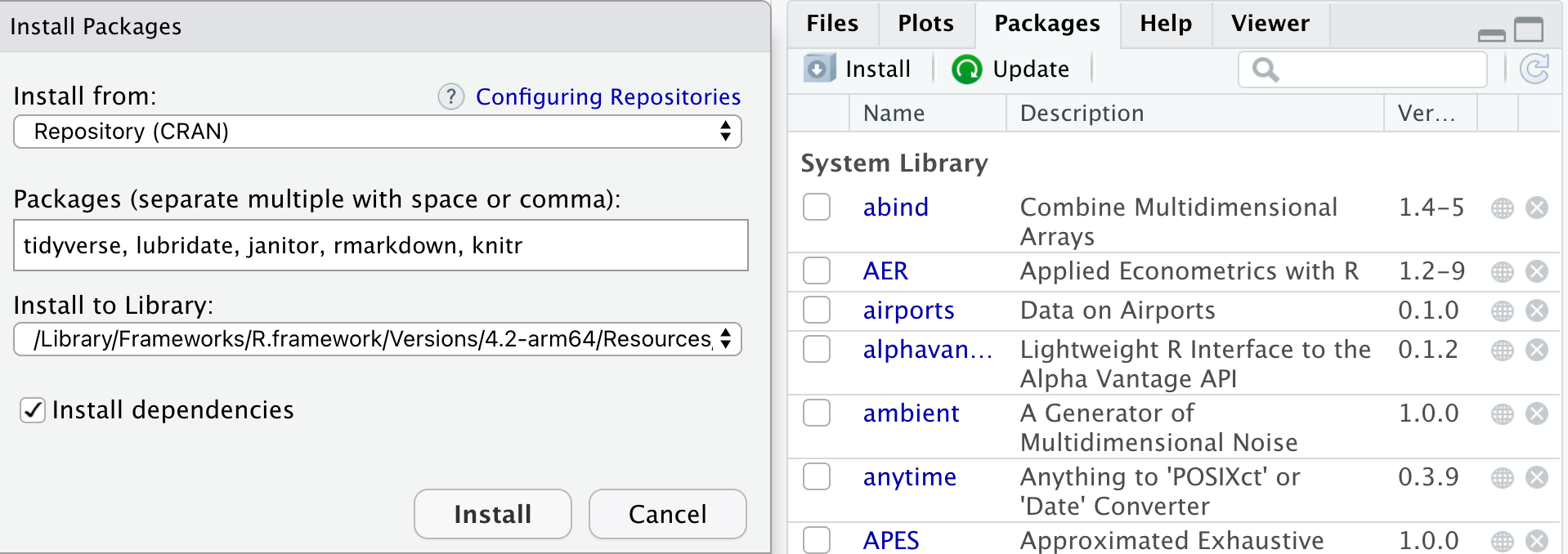
If you go to the packages pane, you should see some packages already installed from base R. You can also use install.packages(“package_name_here”) in the console to accomplish the same thing. Here I’ve typed in a few packages that I recommend and you should install first.

A couple of other packages I recommend and why:

• devtools: helps you install packages from Github if they’re not on CRAN
• blogdown: if you want to create a blog like this one
• car (Companion to Applied Regression) and caret (Classification and Regression Training): if you need to build and test regression models
• fuzzyjoin: for situations where you don’t have a key to join different datasets together
• ggeffects: get tidy dataframes of model output for plotting
• ggpubr: offers an easy way to combine plots
• ggthemes: extends the built-in ggplot2 themes to offer more styling
• gtsummary: easy and nicely formatted tables
• flextable: formatting for tables, also allows for gtsummary tables to be knitted to word documents
• officedown and officer: if you have the misfortune of being forced to use Word and PowerPoint in your work
• reactable: interactive data tables for html documents, shiny apps, etc.
• rstatix: great tidy interface to statistical tests, correlations, etc.
• shiny: for interactive dashboards and apps
• tibbletime: time-aware tibbles for time series analysis
• tidymodels: a collection of packages for modeling and machine learning
• writexl: write out excel files, is not java dependent

Using RStudio

Base R has some built-in datasets you can access, so I’ll use the mtcars data to illustrate some more of RStudio’s features. You can see that once I load the dataset, it shows up in the top right panel under Environment. When you click on the arrow next to the dataset name, you’ll see the list of columns and their data types.

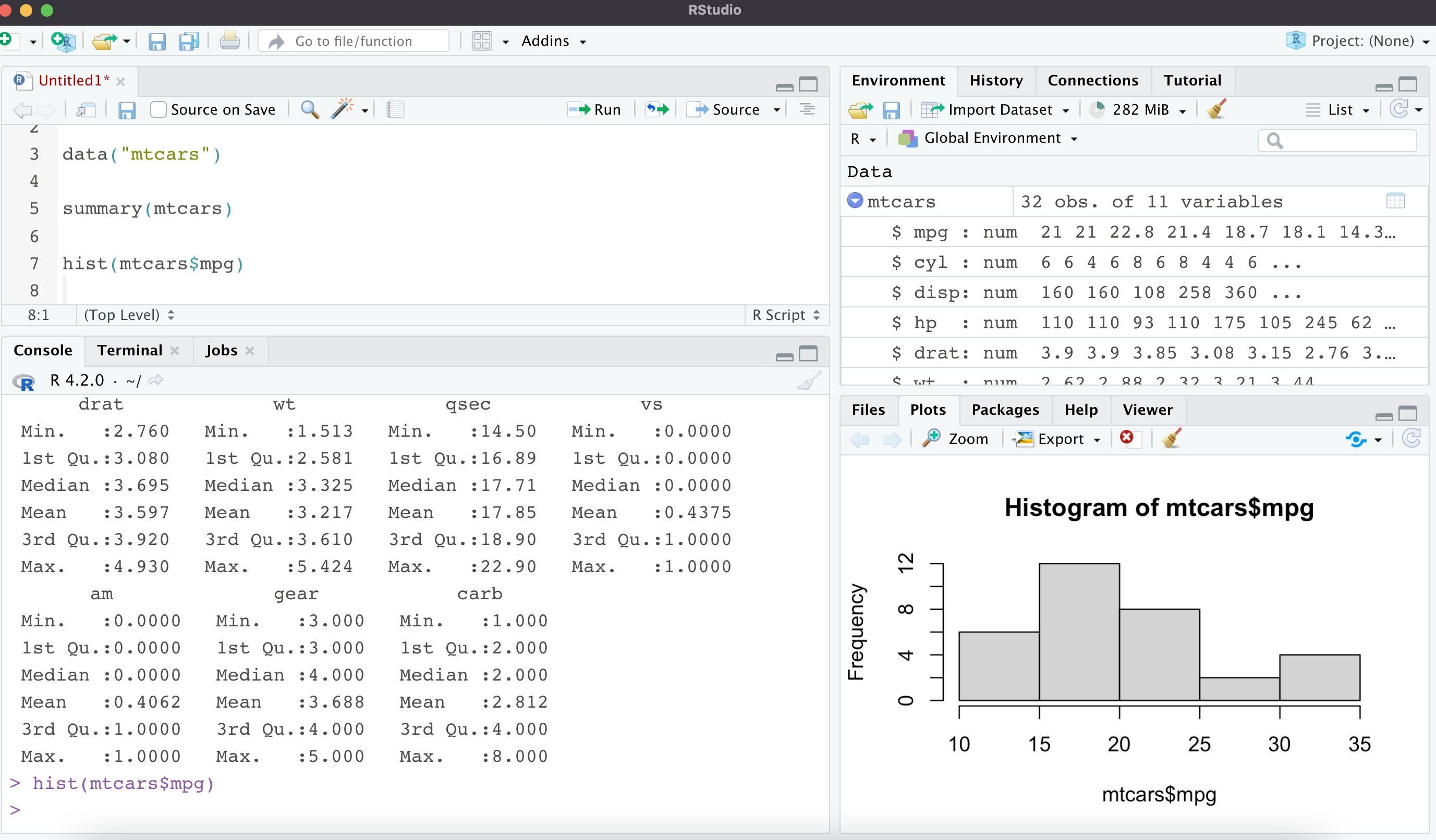
Using the summary() function you can get a quick snapshot of the dataset. This is great for numeric, date, and factor data types. I’ve also used the built-in base R plotting function (hist) to create a histogram of the mpg column, which shows up in the Plots pane on the bottom right.

Exploring Data

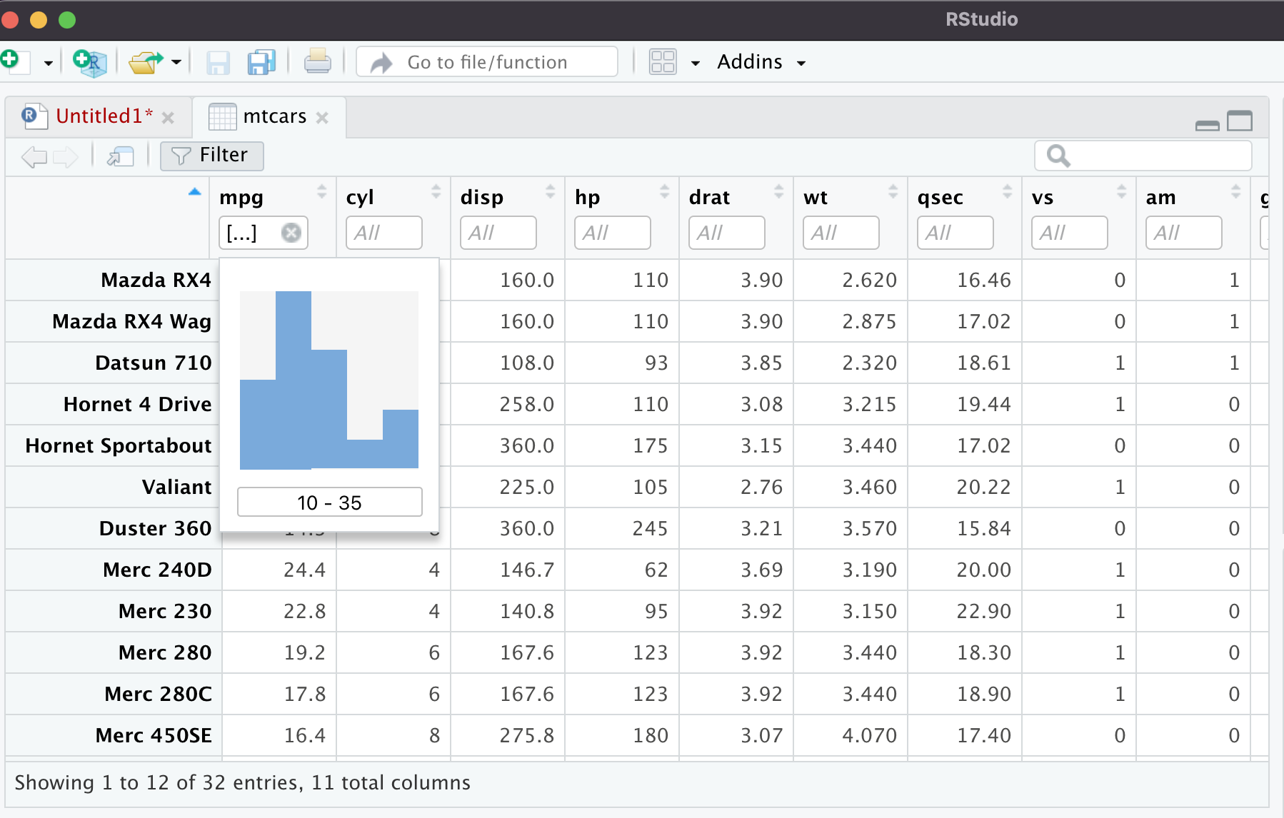
If you click on the mtcars dataset in the Environment pane, it will pop up in the data explorer as a new tab. You can actually sort the data by clicking on the columns, or you can filter it. When I click filter, it brings up a histogram and tells me what the column type is. Under the histogram where it says 10-35, I can type in a number there and it will filter the column. The same thing works for strings/characters, and all the other variable types.

Setting Up an R Project

R Projects can be really convenient for your workflow, as they are an easy way to switch between different analyses. To start a new project, you can go to the Project dropdown at the top right, which currently says “(none)” indicating that we’re just in a regular Rstudio session right now, no project is loaded.

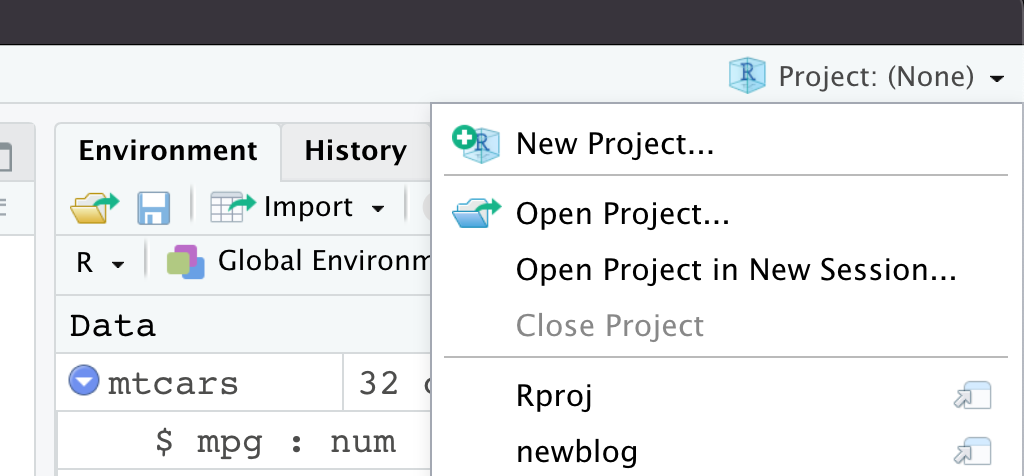
You can also create a new project by going to File -> New Project. Either way, you should get a popup like this:

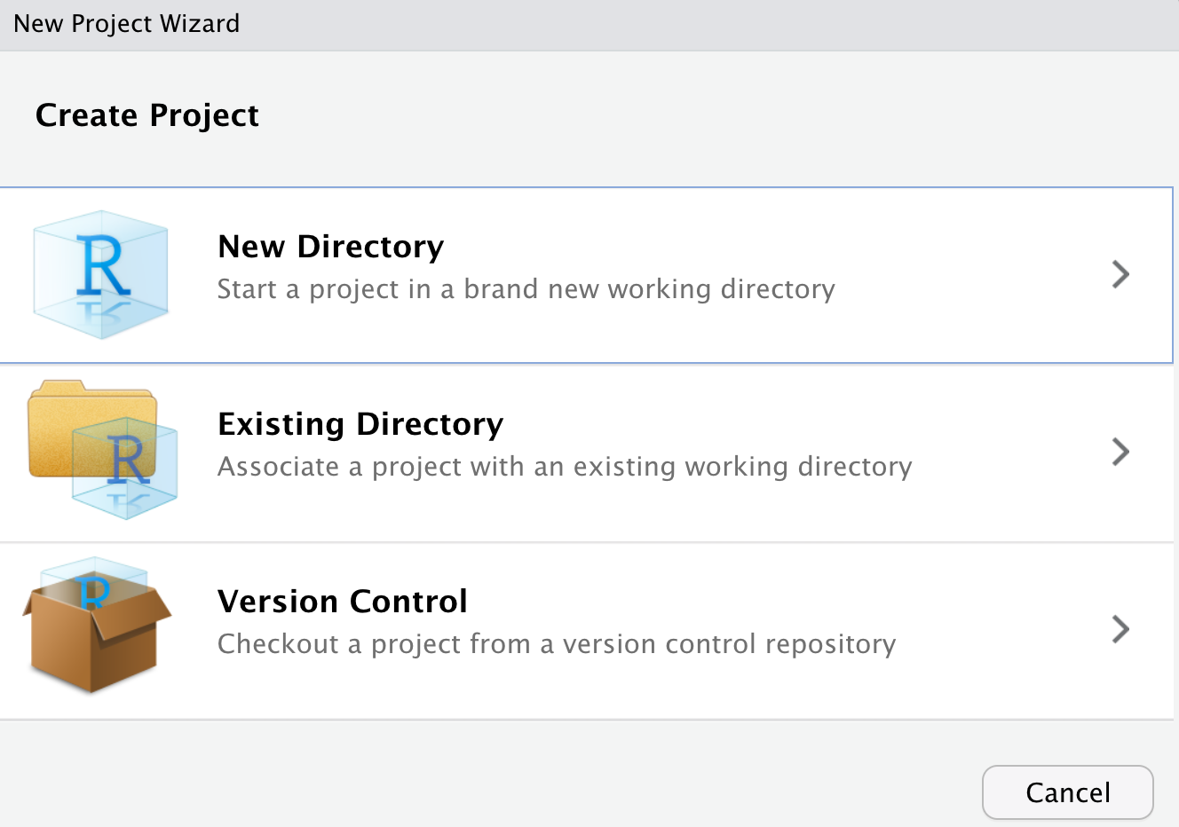
There are three main ways you can create a project. The first two are quite similar - the only difference is with “New Directory” you will create a new folder somewhere on your computer, and with “Existing Directory” you’ll choose a folder that already exists. The third option is to create a project with version control. This is actually quite convenient, you can commit and push to your Github repo right from RStudio. But that’s a topic for another day.

Today I’m going to create an example project on my desktop called “testproject”. Click “new directory”, then “new project”, and you’ll get to this screen:

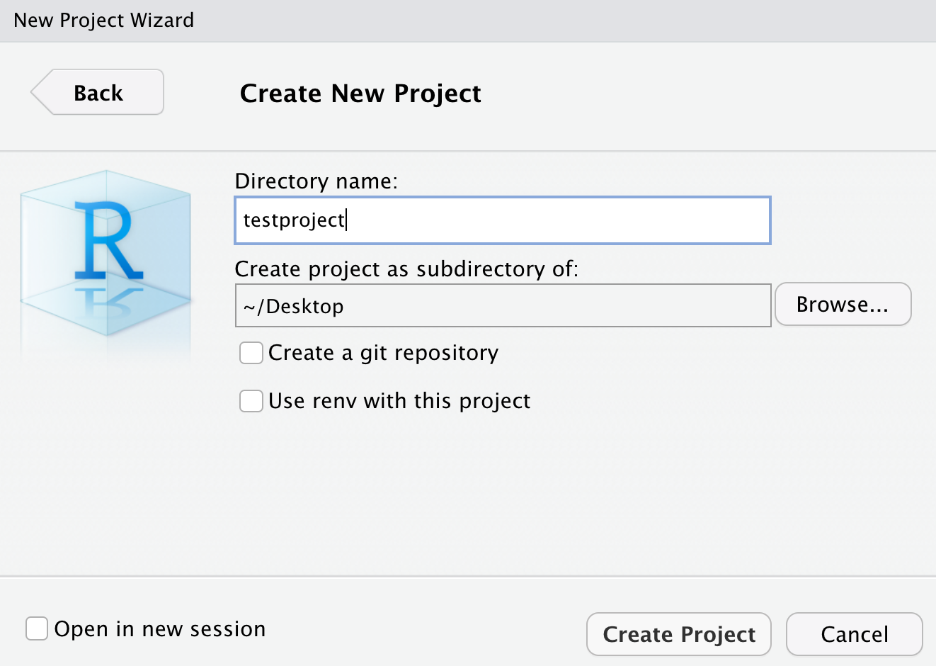
Choose your destination folder or location, and name your project, then click “create project”. Your RStudio should reload, then you’ll see “testproject” at the top right.

Brief Intro to Rmarkdown

I use Rmarkdown documents quite a bit because it’s nice to have all your code and notes in one place. Go to File -> New File -> R Markdown and you’ll get this popup window.

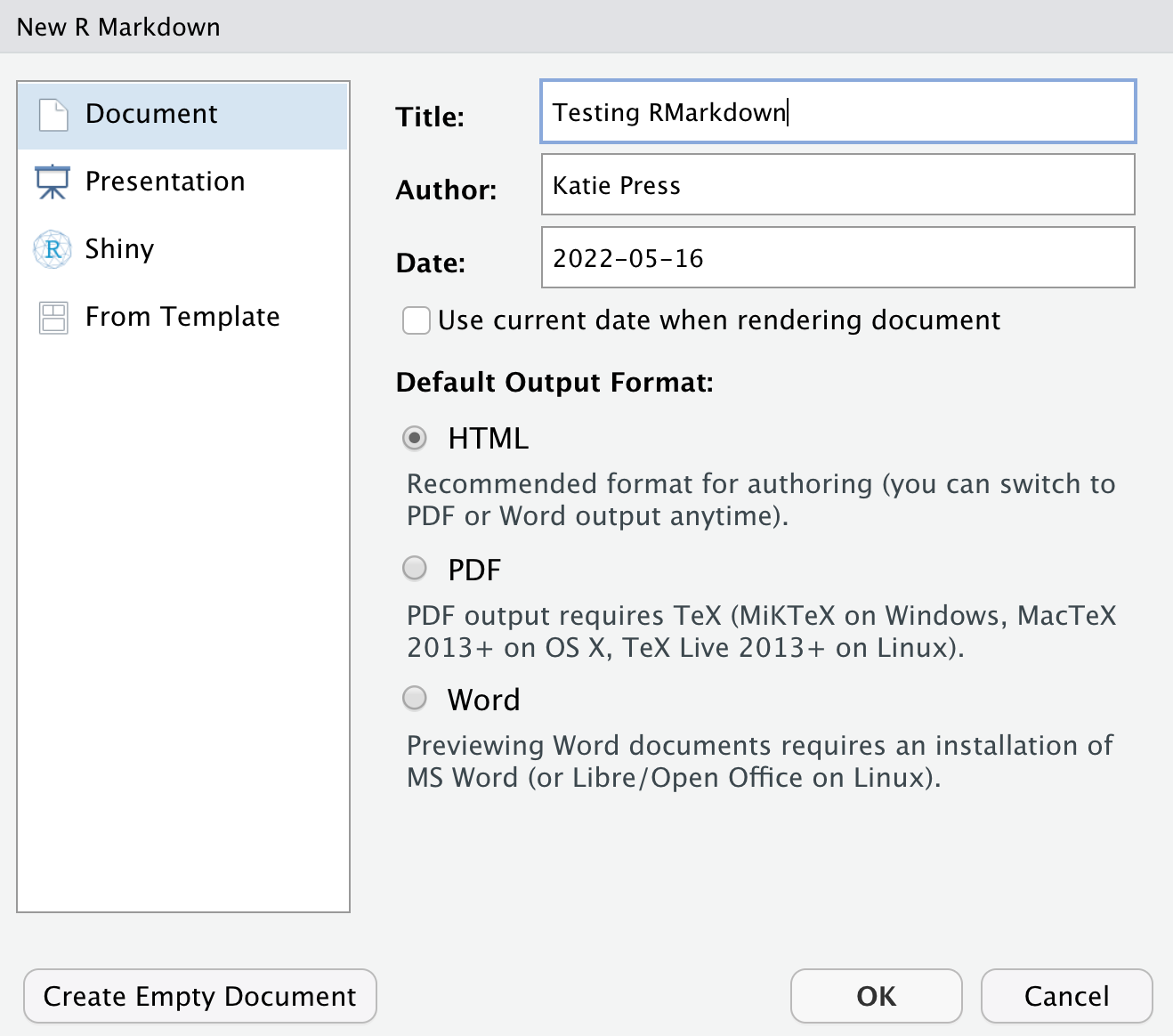
You don’t need to worry about all the other stuff for now, but there are lots of options, including PowerPoint presentations, lightweight dashboards, Shiny apps, and more. We’re just going to use a default html Rmarkdown document. Name your document and click “okay”. You should see some pre-filled example content in your new document. You can try knitting it and see what happens.

RMarkdown Document Structure

The Rmarkdown document has some important components which I’ve annotated with arrows. The YAML header is the starting place for the document format. It specifies what type of document the output will be (in this case, html), it adds the author name, date, and title to the document, and there are many other features that you can use depending on the document type you choose. For example, in an html document we could add a table of contents, make it float on the page so that it follows the reader as they scroll, and specify what header levels to include in the table of contents. Not all features are available in all document types. I recommend checking out the R Markdown Cookbook for more information.

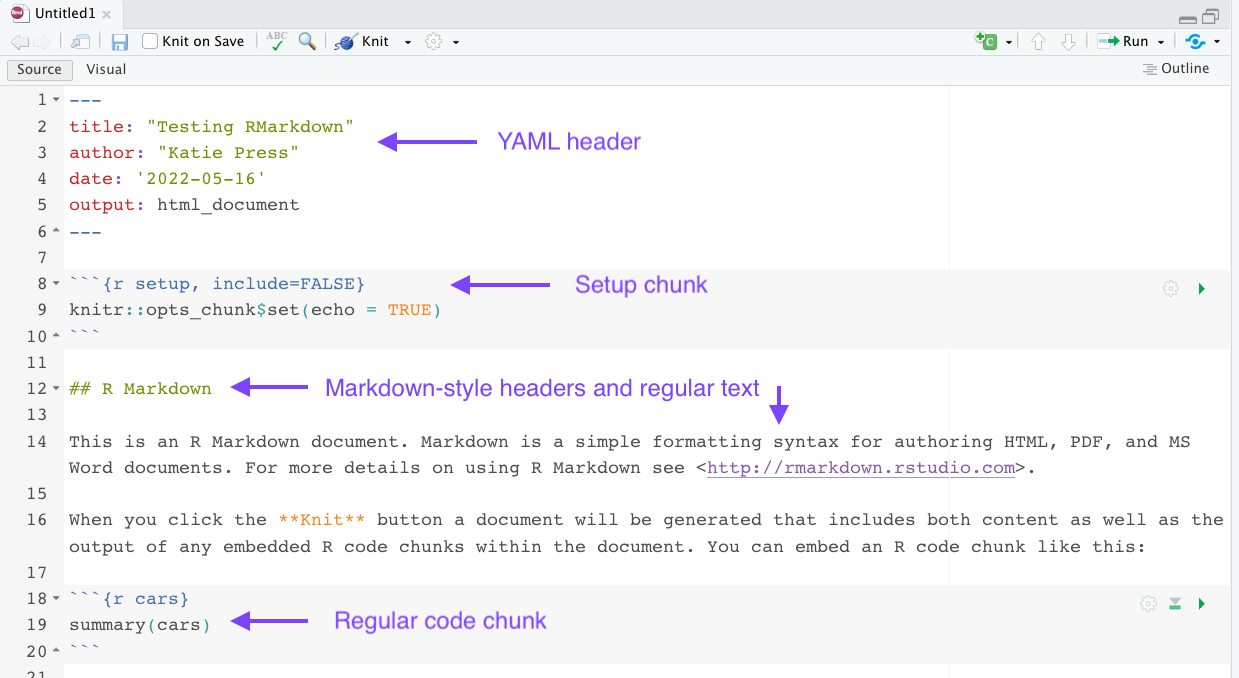
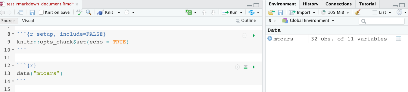
The setup chunk is where you should load your packages. One benefit to doing it this way is that the setup chunk will run automatically first if you try and run any other code chunk. in the knitr::opts_chunk$set you will be able to set formatting for the entire document. The example code here has echo = TRUE. This means that the code chunks will be shown in the resulting knitted document, and this will apply to all chunks in the document. You can still override it in individual chunks if you want.

Just like in regular Markdown documents, you can use hashtags to designated header levels. I often start with header level 2 just because the largest one can be overly large. You can write normal text outside of the code chunks just like you would in any other word processing document.

Using Code Chunks

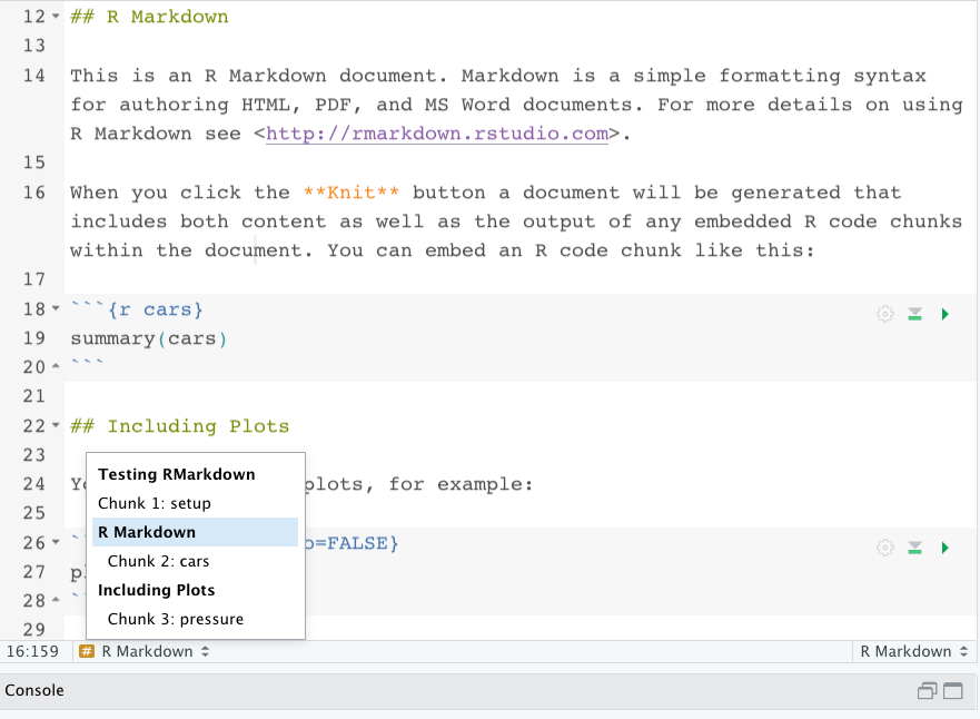
Finally, you can see the regular code chunk at the bottom which doesn’t have as much information in it as the setup chunk. It does have an “r” in it, you need that to evaluate r code. The “cars” is just naming that chunk so you can find it easily in your Rmarkdown document outline. You can find this at the bottom of your RStudio just above the console. As you can see from the screenshot below, the outline includes your markdown headers as well as the names of the code chunks. You don’t have to name them, if you leave them blank they will be numbered instead.

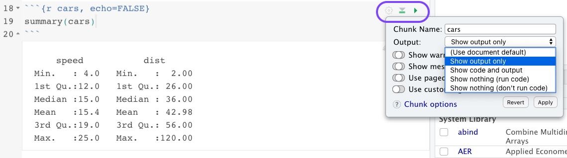
If you click the arrow on the far right-hand side of the code chunk, the code will run “in-line”, which pops up a little output window right in the document instead of in the console or a plot window. You should be able to hit command+enter if you have your cursor in the code chunk to run it as well. The next arrow to its left will allow you to run all chunks above or below your current chunk. You can click on the gear symbol to set the specifications for one chunk in particular, or you can just write them inside of the curly braces, separated by commas. For example, if I choose “show output only”, it adds “echo=FALSE” to the code chunk. That means you will see the output of speed and dist below, but you won’t see the code chunk containing “summary(cars)” in the resulting html document.

Knitting a Document

When you’re ready to knit your document, all you have to do is click on the little yarn ball up at the top. If you click on the arrow next to it, you’ll get a dropdown with a few more options. If I choose “Knit to HTML”, it will simply knit the document, because our YAML header already specifies that it’s an html doc. However, if I choose “Knit to PDF”, it doesn’t change the document type but it will actually add a PDF document and output both at once.

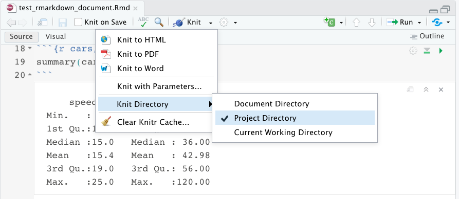
One other important feature I wanted to highlight is the knit directory. This specifies where the knitted document will be saved in your folder structure. If you choose document directory, it will be saved right alongside the Rmarkdown document, wherever that is saved. If you choose project directory, it will be saved in your overall project folder. If you’re working in an R project, these locations might be the same. But maybe you have a lot of files and you want to keep your folder structure more organized.

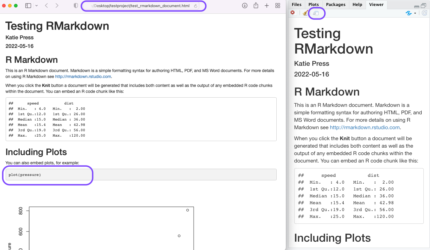
So I’ve knitted my document, and it popped up in my “Viewer” pane on the right. If I click the little dataframe with the arrow icon, it will open it up in a browser window. Note that this is not currently published anywhere, it only exists on your computer. Also notice I changed the plot chunk to “echo=TRUE” so that the code chunk will show up, unlike the summary(cars) code chunk above which I set to “echo=FALSE”.

Organizing and Saving Your R Project

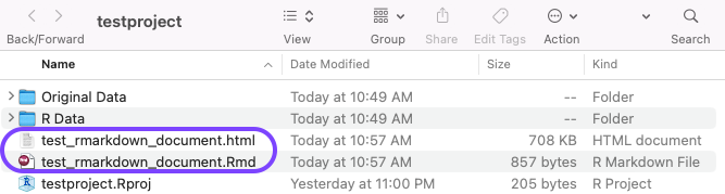
Okay, back to what I was saying about the knit directory. Here is an example of what my folder structure looks like now that I knitted the first RMD document. You can see that the .Rmd file and the html output are both here in my project directory. RIght above that are two subfolders that I added. I like to keep my original data in one folder, and R data/cleaned data in another folder. Reading and writing out data will be in the next tutorial.

Just below the purple box is the testproject.Rproj. When you exit out of your R Project, this is where your workspace is going to be saved. To illustrate how this works, I’m going to load the mtcars dataset again. I like to load my data in a separate code chunk right under the setup chunk where I load the packages. When you run data(“mtcars”) you might see something that says “” in your environment pane. The minute you actually try to use the dataset in any way—for example, running summary()—it will pop up as an actual dataframe.

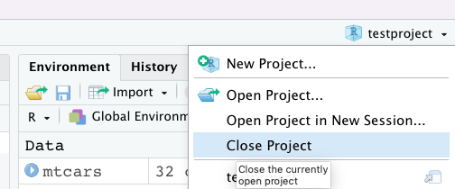
So at this point, I have an .Rmd doc and a dataset loaded in my project. If I quit out of RStudio, or close the project like so:

I will get a popup that looks like this:

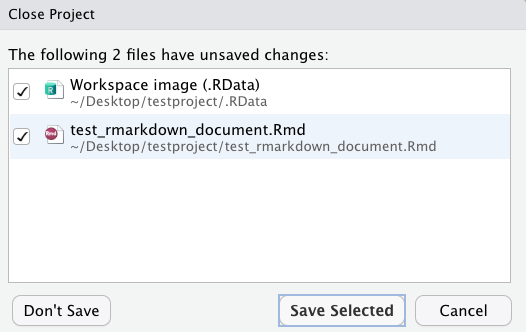
I hadn’t saved my RMD doc since adding the mtcars data, so it shows up in this window along with my overall project workspace. I want to click “save selected”, and it will exit out of the project. Next time I want to use this project, I can either open up my RStudio first and open the project from the file menu and my list of recent projects, or I could simply click on the testproject.Rproj icon in my folder on my desktop and it would open up RStudio for me. Either way, this is what I see when I open up the project again:

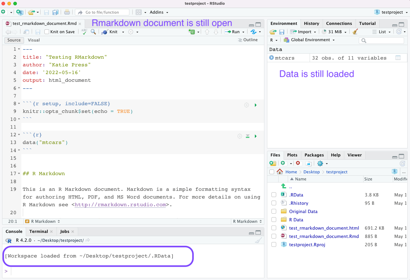
RStudio and Rmarkdown have many more useful features that I will discuss in other tutorials. Hopefully this was a helpful intro to RStudio.