Tidy Tuesday: Du Bois Challenge 2022
By Katie Press in TidyTuesday
February 15, 2022
Overview
This week’s Tidy Tuesday challenge is a collaboration with the #DuboisChallenge2022. One of the things I love about Du Bois’ data visualizations is that he used them to highlight the achievements and culture of Black Americans in addition to the struggles they faced. I own the book W.E.B Du Bois’s Data Portraits Visualizing Black America and I thought I would share the summary from the back of the cover:

“At the 1900 Paris Exposition, the famed sociologist and civil rights activist W.E.B Du Bois presented a series of groundbreaking data visualizations advocating for African American progress. These graphs, charts, and maps provided powerful glimpses into the lives of black Americans to convey both a literal and figurative representation of what Du Bois famously referred to as “the color line”. From advances in education to the lingering effects of slavery, these infographics—beautiful in design and impactful in content—made visible a wide spectrum of black experience.”
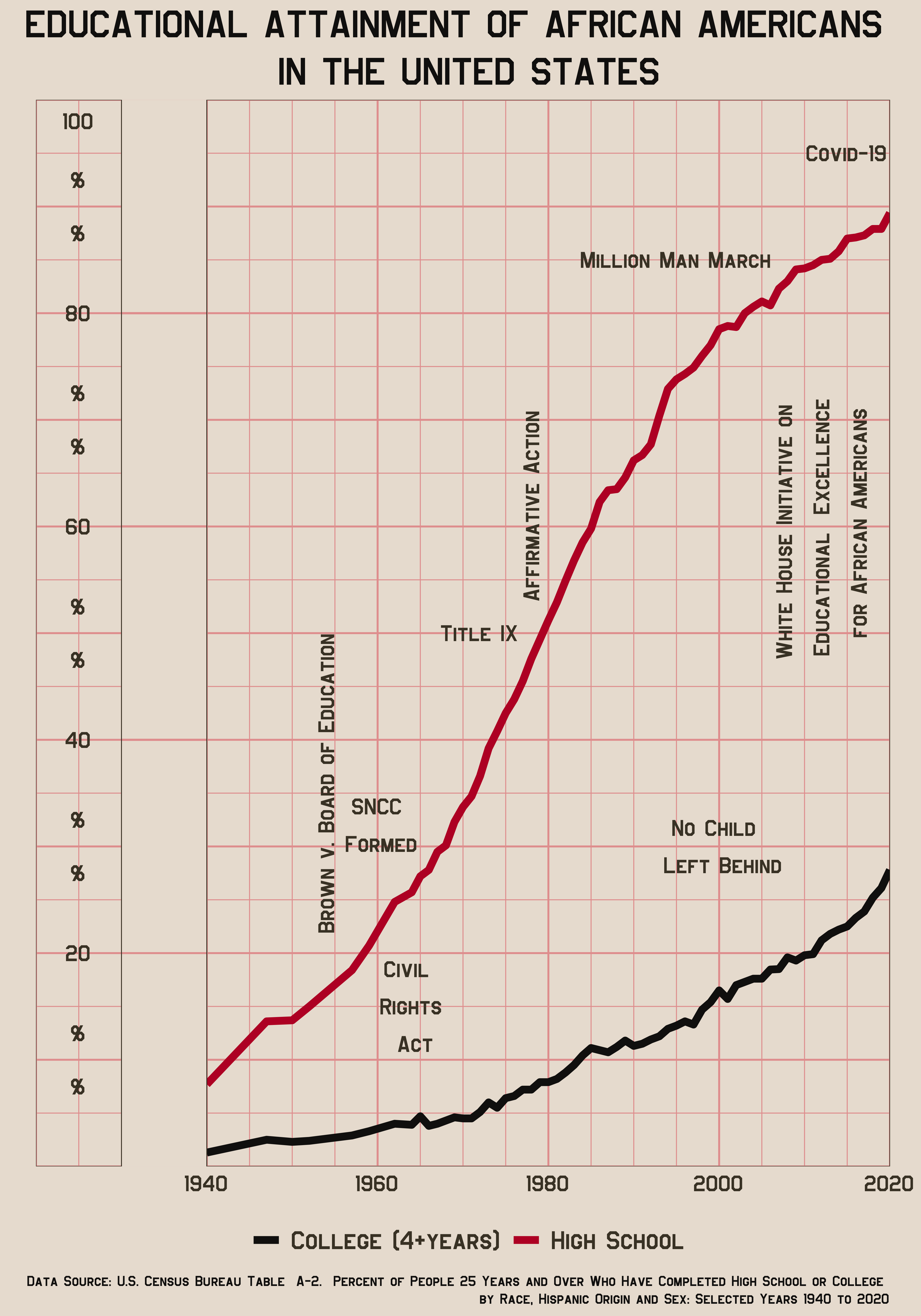
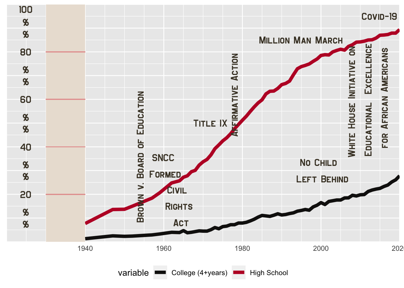
With that in mind, I decided to focus on educational advances in more recent history using census data. My new version of the chart is on the left, and the chart I used for inspiration is on the right:
| New DuBois Chart | Original DuBois Chart |
|---|---|
 |
 |
Data
I retrieved this data from the U.S. Census historical tables and decided to copy and paste what I wanted into another sheet as opposed to reading it into R and trying to clean it up. I’ve done that before, but this is not a lot of data and sometimes you just have to work smarter not harder. I’ve also uploaded it to Kaggle.
data <- read_excel("/Users/katiepress/Desktop/Rproj/DuboisChallenge/race_education_data.xlsx",
    sheet = "clean_data") %>% clean_names()
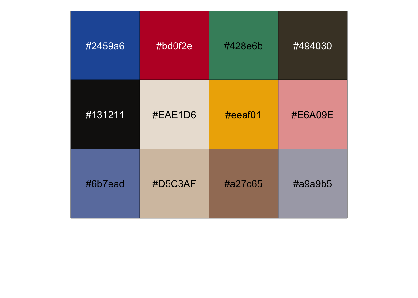
Color Palette
I used coolors.co to create my color palette. They have an image upload feature and it’s really easy to find complementary colors in the generator as well. I knew I probably wouldn’t use them all on this chart, but I might create more for the Dubois Challenge soon.
dark.blue <- "#2459a6"
dark.red <- "#bd0f2e"
dark.green <- "#428e6b"
dark.brown <- "#494030"
light.tan <- "#EAE1D6"
dark.yellow <- "#eeaf01"
dark.black <- "#131211"
light.pink <- "#E6A09E"
light.blue <- "#6b7ead"
medium.brown <- "#a27c65"
light.brown <- "#D5C3AF"
pale.blue <- "#a9a9b5"


scales::show_col(c(dark.blue, dark.red, dark.green, dark.brown, dark.black, light.tan, dark.yellow, light.pink, light.blue, light.brown, medium.brown, pale.blue))
I’m going to set a few color values for the charts so if I want to change something, I only have to updated it here and not a bunch of different places.
background.color <- light.tan
hline.color <- light.pink
linecol.1 <- dark.black
linecol.2 <- dark.red
grid.color <- light.pink
text.annotate.color <- dark.brown
annotation.size <- 5
Creating the Chart
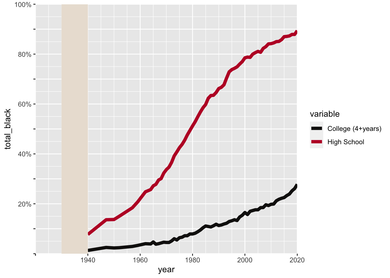
First I will create a line chart of the overall percentages of high school and college educated African Americans over time. I’m taking some liberties with the colors here because I want to use two different lines instead of one like the original chart I’m using for inspiration.
I’m being strategic about the axis breaks and labels - I want to create enough space for everything but I only want certain years to be labeled. I also needed to use expand inside the scales to make sure the grid doesn’t extend beyond the panel so I can keep the same look as the original chart. I briefly considered creating two plots and arranging them in a grid because of the split between the scale and the grid in the original plot. But I realized that was going to be too annoying, and thought of an easier way - using geom_rect. The first draft looks very ugly, but it will improve from here.
plot <- data %>%
  filter(!is.na(year)) %>%
  mutate(total_black = total_black / 100) %>%
  select(variable, year, contains("_black")) %>%
  ggplot(aes(x = year, y = total_black, color = variable)) +
  geom_line(size = 2) +
  scale_color_manual(values = c(linecol.1, linecol.2)) +
  scale_y_continuous(
    limits = c(0, 1),
    labels = c("", "", "20%", "", "40%", "", "60%", "", "80%", "", "100%"),
    breaks = seq(0, 1, .1),
    minor_breaks = seq(0, 1, .05),
    expand = c(0, 0)
  ) +
  scale_x_continuous(
    limits = c(1920, 2020),
    breaks = c(1920, 1940, 1960, 1980, 2000, 2020),
    minor_breaks = seq(1920, 2020, 5),
    expand = c(0, 0),
    labels = c("", "1940", "1960", "1980", "2000", "2020")
  ) +
  annotate(
    "rect",
    xmin = 1930,
    xmax = 1940,
    ymin = 0,
    ymax = 1,
    fill = background.color
  )

plot
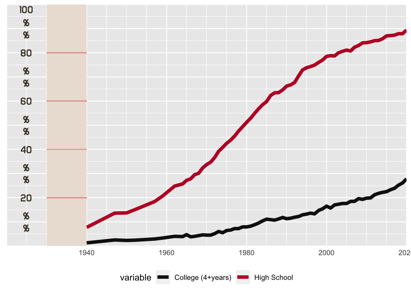
Add Horizontal Lines
I’m using geom_segment to add the horizontal lines to “connect” what will look like two different portions of the chart in the end. Then I’ll add geom_text to replace the y-axis. I would have just used hjust in the axis theme but for some reason the “100” at the top was skewed to the side instead of being centered like the other numbers. I tried expanding the grid limit just a bit over 0 on the y axis but that didn’t work. This was just as well, because I decided to add percentages to resemble the dollar signs in the original chart. I’m using the font “Jeffries” which is part of the themedubois package, but extrafont wasn’t working for me for some reason, so I’ve downloaded the free font and added it to my local font book.
plot <- plot+
  geom_segment(x = 1930, y = .2, xend = 1940, yend = .2, color = hline.color)+
  geom_segment(x = 1930, y = .4, xend = 1940, yend = .4, color = hline.color)+
  geom_segment(x = 1930, y = .6, xend = 1940, yend = .6, color = hline.color)+
  geom_segment(x = 1930, y = .8, xend = 1940, yend = .8, color = hline.color)+
  annotate(
    "text",
    x = 1925,
    y = c(.2, .4, .6, .8, .98),
    label = c("20", "40", "60", "80", "100"),
    color = text.annotate.color,
    size = annotation.size,
    family = "Jefferies"
  ) +
  annotate(
    "text",
    x = 1925,
    y = c(.075, .125, .275, .325, .475, .525, .675, .725, .875, .925),
    label = "%",
    color = text.annotate.color,
    family = "Jefferies",
    size = annotation.size
  ) +
  theme(
    axis.ticks = element_blank(),
    axis.text.y = element_blank(),
    axis.title = element_blank(),
    legend.position = "bottom"
  )

plot
Add annotations for historical events.
Right now it’s going to look like the text is way too large, but I’m going to make the entire plot size larger in a minute.
plot <- plot +
  annotate("text", x = 1954, y = .36, label = "Brown v. Board of Education",
    color = text.annotate.color,
    family = "Jefferies",
    size = annotation.size, angle = 90)+
  annotate("text", x = 1960, y = .32, label = " SNCC \n Formed",
    color = text.annotate.color,
    family = "Jefferies",
    size = annotation.size)+
  annotate("text", x = 1964, y = .15, label = "Civil \n Rights \n Act",
    color = text.annotate.color,
    family = "Jefferies",
    size = annotation.size)+
  annotate("text", x = 1972, y = .5, label = "Title IX",
    color = text.annotate.color,
    family = "Jefferies",
    size = annotation.size)+
  annotate("text", x = 1978, y = .62, label = "Affirmative Action",
    color = text.annotate.color,
    family = "Jefferies",
    size = annotation.size, angle = 90)+
  annotate("text", x = 2000, y = .3, label = "No Child \n Left Behind",
    color = text.annotate.color,
    family = "Jefferies",
    size = annotation.size)+
  annotate("text", x = 2012, y = .6, label = "White House Initiative on \n Educational  Excellence \n for African Americans",
    color = text.annotate.color,
    family = "Jefferies",
    size = annotation.size, angle = 90)+
  annotate("text", x = 2015, y = .95, label = "Covid-19",
    color = text.annotate.color,
    family = "Jefferies",
    size = annotation.size)+
  annotate("text", x = 1995, y = .85, label = "Million Man March",
    color = text.annotate.color,
    family = "Jefferies",
    size = annotation.size)

plot
Styling
I added a title and a caption for the data source. At this stage, I’m making the background a uniform color and changing the grid lines to light red. I realized at the last minute I also needed to make the grid panel outline a darker color, so I added more geom_segments for that. I would usually use the panel.background color in the theme, plus maybe the outline color of the geom_rect I used to separate the two pieces of the plot. But I couldn’t do that and remain true to the original, because there are no lines across the top in the original. This is obviously not the most efficient way of doing things, but again I’m going for style here.
After adding the rest of the theme elements, things are finally starting to come together here, it just needs to be resized.
plot <- plot+
  ggtitle("EDUCATIONAL ATTAINMENT OF AFRICAN AMERICANS \n IN THE UNITED STATES")+
  labs(caption = "Data Source: U.S. Census Bureau Table  A-2.  Percent of People 25 Years and Over Who Have Completed High School or College \n by Race, Hispanic Origin and Sex: Selected Years 1940 to 2020")+
  geom_segment(x = 1940, y = 0, xend = 1940, yend = 1, color = dark.brown, size = .15)+
  geom_segment(x = 1930, y = 0, xend = 1930, yend = 1, color = dark.brown, size = .15)+
  geom_segment(x = 1920, y = 0, xend = 1920, yend = 1, color = dark.brown, size = .15)+
  geom_segment(x = 2020, y = 0, xend = 2020, yend = 1, color = dark.brown, size = .15)+
   geom_segment(x = 1920, y = 0, xend = 1930, yend = 0, color = dark.brown, size = .15)+
  geom_segment(x = 1940, y = 0, xend = 2020, yend = 0, color = dark.brown, size = .15)+
  geom_segment(x = 1920, y = 1, xend = 1930, yend = 1, color = dark.brown, size = .15)+
  geom_segment(x = 1940, y = 1, xend = 2020, yend = 1, color = dark.brown, size = .15)+
  theme(plot.background = element_rect(fill = background.color, color = background.color),
        panel.background = element_rect(fill = background.color),
        #panel.border = element_rect(color = dark.brown, fill =NA),
        panel.grid = element_line(color = grid.color),
        legend.position = "bottom",
        legend.title=element_blank(),
        legend.background = element_rect(background.color),
        legend.key = element_rect(fill = NA),
        legend.text = element_text(color = text.annotate.color, family = "Jefferies", size = 16),
        axis.text.x = element_text(color = text.annotate.color, family = "Jefferies", size = 14),
        plot.margin=unit(c(.2,.6,.2,.6),"cm"),
        plot.title = element_text(size = 24, color = dark.black, family = "Jefferies", hjust = .5),
        plot.caption = element_text(size = 9, family = "Jefferies", color = dark.black)
        )

plot
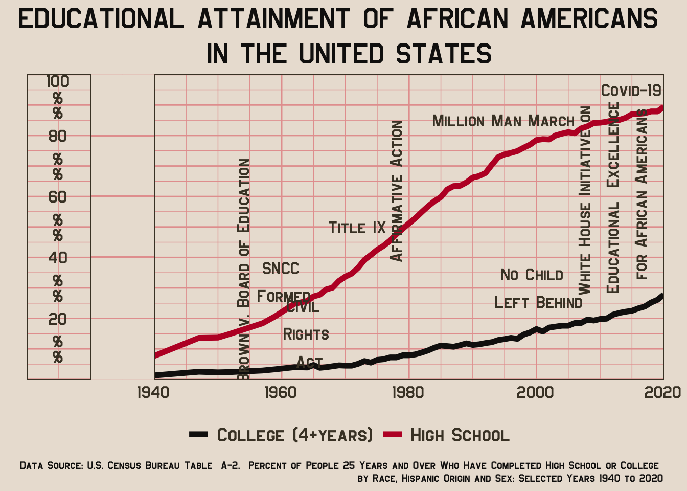
Final Sized Plot
Here’s the final result! This chunk uses fig.width=7, fig.height=10, dev=‘png’, dpi=300. It can be saved as a png using the same specifications with ggsave().