Replacing the Magrittr Pipe With the Native R Pipe

What’s the deal with the new pipe?

R version 4.0+ has a “native” pipe |> that does not rely on the magrittr dependency. Apparently it is supposed to be faster than the magrittr pipe, which does a lot more “behind the scenes”. You can read more about it in R for Data Science. There are also a couple of other blog posts out there on the subject. I decided to give it a go since I like to try new things, so I decided to run a bunch of my old code, just replacing the old pipe with the native pipe to see what would happen. Surprisingly I had very few issues, but I thought I would write this blog posts describing the couple times where it did fail, and how I fixed it.

knitr::opts_chunk$set(echo = TRUE)
library(esvis)
library(tidyverse)
library(rvest)
library(janitor)

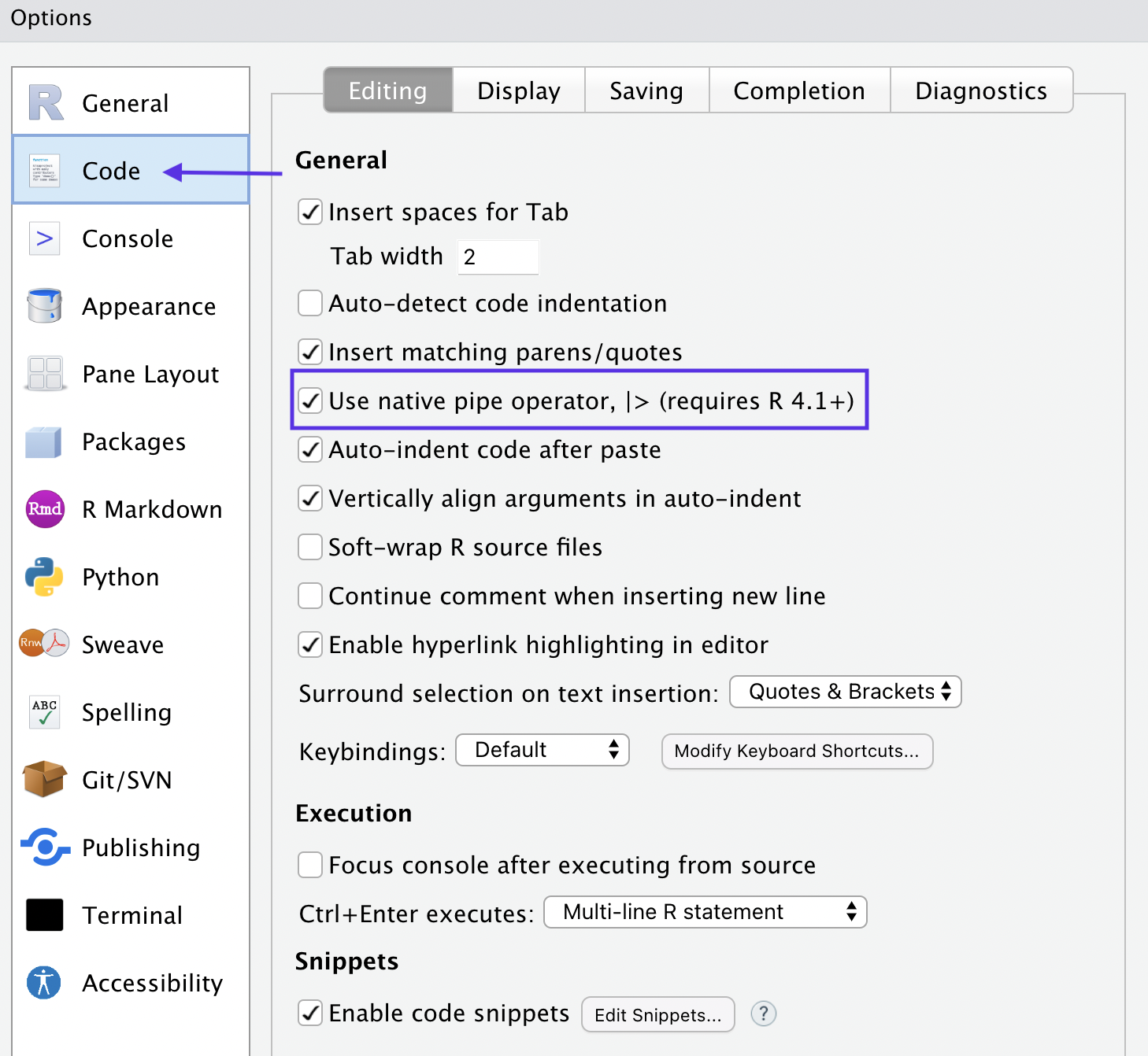
First of all, you can change your shortcut to the native pipe operator through the global settings under “code” like so:

There are some differences to be aware of when using the native pipe - primarily that it doesn’t work with dot notation. You have to use an anonymous function instead, which I will illustrate in the three examples in this post.

Example 1: mapping to clean names

I don’t want to load all the data necessary for this example, so here’s a quick list of dataframes to use.

data_list <- list(
  data1 = tibble(Var1 = c("a", "b", "c"), `Variable #2` = c(1,2,3)),
  data2 = tibble(Var1 = c("a", "b", "c"), `Variable #2` = c(1,2,3))
)

This code did not work when I replaced it with the native pipe.

data_list %>%
  map( ~.x %>% clean_names)

Again, it just needed to be replaced with an anonymous function. This time I’ve used x instead of the dot so you can see it still works.

data_list |> 
  map(\(x) clean_names(x))

## $data1
## # A tibble: 3 × 2
##   var1  variable_number_2
##   <chr>             <dbl>
## 1 a                     1
## 2 b                     2
## 3 c                     3
## 
## $data2
## # A tibble: 3 × 2
##   var1  variable_number_2
##   <chr>             <dbl>
## 1 a                     1
## 2 b                     2
## 3 c                     3

Example 2: The native pipe doesn’t work with split and dot notation

The first code failure is from a file I created for someone who asked how they could map over several variables when testing effect sizes. This is really just an example to show the features of purrr. I’m using example data from the esvis package.

data(star)

star <- star |> 
  select(condition, sex, reading) |> 
  gather(variable, value, - reading)

This was my original code, and when I replaced the magrittr pipe with the native pipe it didn’t work.

star %>%
  split(.$variable) %>%
  map_df(. %>% hedg_g(., reading ~ value), .id = "variable")

The native pipe does not allow the use of the period placeholder with the dollar sign, or with brackets for that matter which we’ll see in a minute. But the tilde works to split by variable, and then I just had to replace the dot notation with an anonymous function instead. It doesn’t have to use the dot, you could replace it with x or whatever name you want.

star |> 
  split(~variable) |> 
  map_df(\(.) hedg_g(., reading ~ value), .id = "variable")

## # A tibble: 8 × 5
##   variable  value_ref value_foc   coh_d  hedg_g
##   <chr>     <chr>     <chr>       <dbl>   <dbl>
## 1 condition reg       reg_aid    0.0258  0.0258
## 2 condition reg       small     -0.159  -0.159 
## 3 condition reg_aid   reg       -0.0258 -0.0258
## 4 condition reg_aid   small     -0.186  -0.186 
## 5 condition small     reg        0.159   0.159 
## 6 condition small     reg_aid    0.186   0.186 
## 7 sex       boy       girl      -0.193  -0.193 
## 8 sex       girl      boy        0.193   0.193

Example 3: Using the native pipe while accessing data with brackets

Remember I said the base pipe would not allow the dot notation with brackets? This is an example of the code I tried to run which didn’t work when I just replaced the pipe.

wiki <- "https://en.wikipedia.org/wiki/Dow_Jones_Industrial_Average"

djia <- wiki %>% 
  read_html() %>% 
  html_nodes("table") %>% 
  .[[2]] %>% 
  html_table(fill = TRUE) %>% 
  clean_names()

This one took me a minute to figure out. I had to encase the entire line in parentheses, use the anonymous function, and then add extra empty parentheses at the end of the line. But it worked!

wiki |> 
  read_html() |> 
  html_nodes("table") |> 
  (\(.) .[[2]])() |> 
  html_table(fill = TRUE) |> 
  clean_names()

## # A tibble: 30 × 7
##    company          exchange symbol industry    date_added notes index_weighting
##    <chr>            <chr>    <chr>  <chr>       <chr>      <chr> <chr>          
##  1 3M               NYSE     MMM    Conglomera… 1976-08-09 "As … 2.88%          
##  2 American Express NYSE     AXP    Financial … 1982-08-30 ""    3.56%          
##  3 Amgen            NASDAQ   AMGN   Biopharmac… 2020-08-31 ""    4.88%          
##  4 Apple            NASDAQ   AAPL   Informatio… 2015-03-19 ""    3.15%          
##  5 Boeing           NYSE     BA     Aerospace … 1987-03-12 ""    3.40%          
##  6 Caterpillar      NYSE     CAT    Constructi… 1991-05-06 ""    4.19%          
##  7 Chevron          NYSE     CVX    Petroleum … 2008-02-19 "Als… 3.05%          
##  8 Cisco            NASDAQ   CSCO   Informatio… 2009-06-08 ""    1.00%          
##  9 Coca-Cola        NYSE     KO     Drink indu… 1987-03-12 "Als… 1.28%          
## 10 Disney           NYSE     DIS    Broadcasti… 1991-05-06 ""    2.32%          
## # … with 20 more rows

Fira code and ligature fonts

Now I’ll write some code just to show you how cool it looks if you use the Fira Code font and enable ligatures. My blog Rmarkdown file will not show the ligatures by default, so the code chunk below is how it would look without Fira Code.

djia |>
  filter(exchange == "NYSE" & company != "3M") |>
  filter(date_added >= "2009-01-01") -> new_djia

And here’s what it looks like in my RStudio console. Pretty cool!

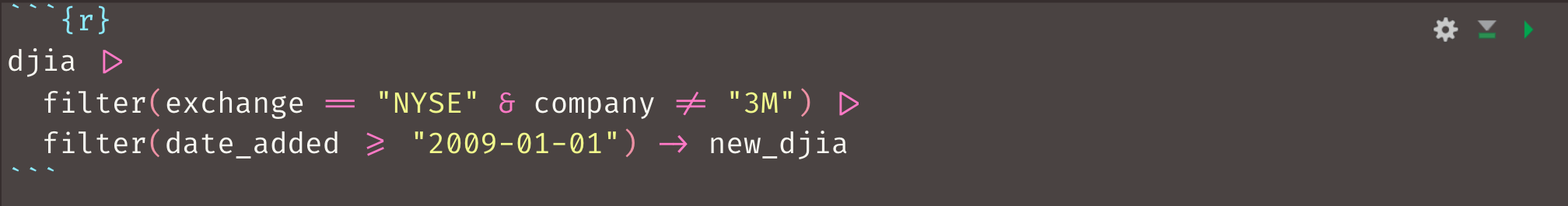
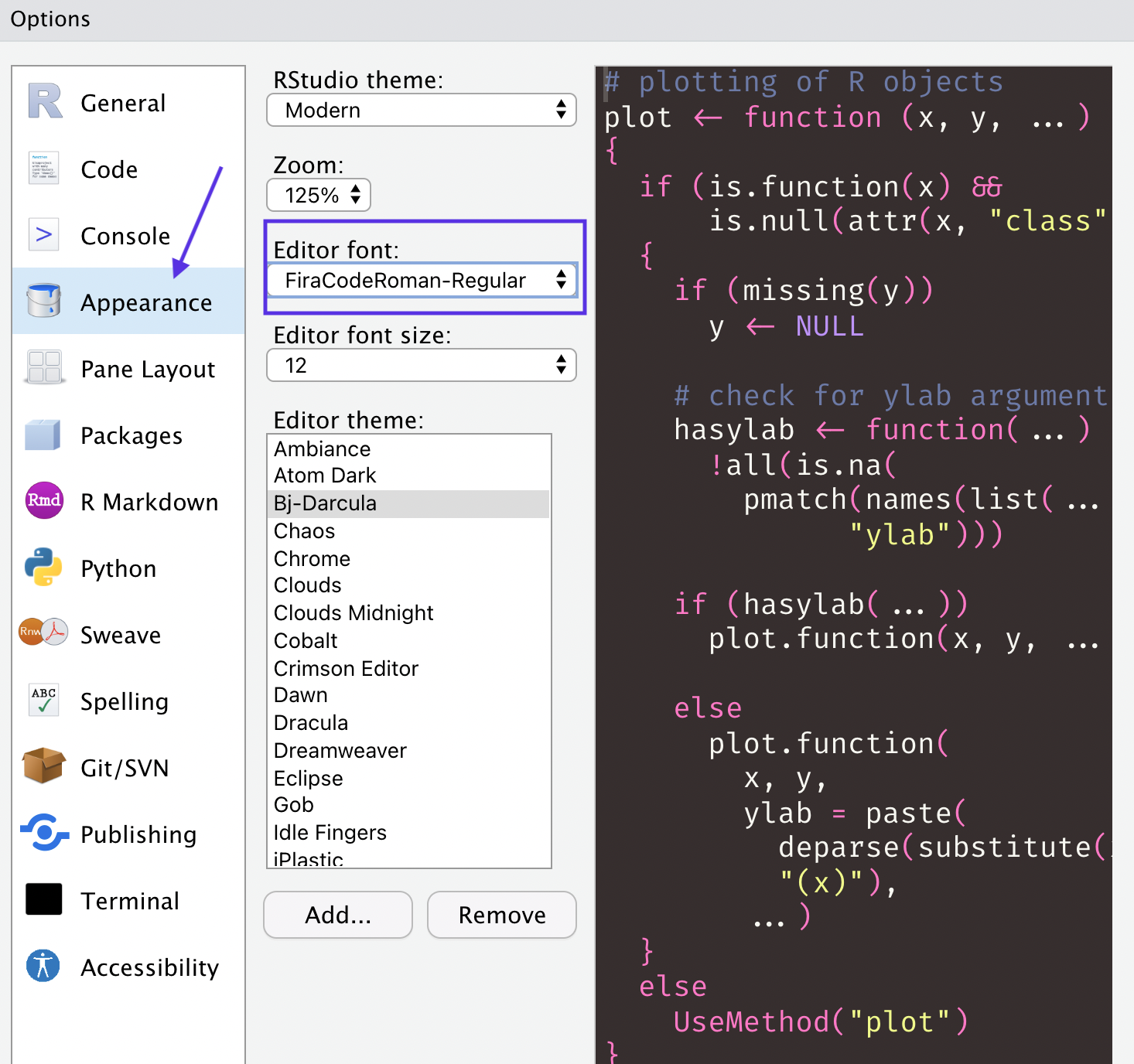
You can do this yourself if you download Fira Code which you can get from Google Fonts. Then go to the global options and change the font settings. Note that you will most likely have to restart RStudio before the font will show up in your list, so don’t worry if you don’t see it there right away.