Tidy Tuesday: Drought Conditions

Data Import and Cleaning

The data provided this week is drought conditions by state. I wanted to make a map, and I thought it would be interesting to look at the drought level by county over time. I downloaded a file from this page on The U.S. Drought Monitor Website

I filtered by date (August 2019 - present), I chose “County” for the spatial scale, “Percent Area” for statistics type, and “Categorical” for statistics type, and downloaded a csv file.

After reading in the csv, I just cleaned it up a bit (similar to the tidytuesday dataset) and then filtered so I have the drought level for the highest percentage area for each county and week.

dr_county <- read_csv("~/Desktop/Rproj/drought_maps/dm_export_20190814_20210714.csv") %>% 
    pivot_longer(cols = None:D4, names_to = "drought_lvl", values_to = "area_pct") %>% 
    janitor::clean_names() %>% 
  mutate(drought_lvl =factor(drought_lvl, levels = c("D4", "D3", "D2", "D1", "D0", "None"))) 


temp_drought <- dr_county %>% 
  group_by(fips, valid_start) %>% 
  arrange(fips, valid_start, desc(area_pct), drought_lvl) %>% 
  slice(1)

This is what the drought data looks like:

Since the drought data has a FIPS code, I can use that to match onto my mapping data (courtesy of the maps package). I need to make the FIPS code a string and pad it with a leading 0 to match the county drought data.

data("county.fips")

county.fips <- county.fips %>% 
  mutate(region = word(polyname, 1, sep = ","),
         subregion = word(polyname, 2, sep = ",")) %>% 
  mutate(subregion = word(subregion, 1, sep = ":")) %>% 
  mutate(fips = str_pad(as.character(fips), side = "left", width = 5, "0"))

Now I can get the USA map and join by FIPS.

map_usa <- map_data("county")

map_usa <- map_usa %>% 
  left_join(county.fips)

## Joining, by = c("region", "subregion")

For some reason the drought data is missing Shannon County, SD, which of course is going to be an issue because it will be a blank space on the map. To deal with that issue, I will first create a time series with tibbletime, then join that to the map data so that each county has a row for each week of the drought data.

series <- tibbletime::create_series("2019-08-20" ~ "2021-07-13", "weekly") %>% 
  mutate(join_col = 1) %>% 
  rename("valid_start" = date)

map_usa <- map_usa %>% 
  mutate(join_col = 1) %>% 
  left_join(series)

## Joining, by = "join_col"

Now I can join the drought data to the map. This should not increase the number of rows in the dataset because it is going to join by week and fips. But there is still the issue of the missing SD county.

To deal with the missing county, I’m basically just going to separate it from the rest of the data temporarily, along with Bennett county, which is right next to Shannon. Then I will use Bennett county to fill in the missing values from Shannon, assuming they are likely to be very similar. Then I will add the rows back to the map_usa data. I’m also recoding the drought level factors because I realized it would be helpful for the map visualization.

map_usa <- map_usa %>% 
  left_join(temp_drought)

## Joining, by = c("fips", "valid_start")

temp_nas <- map_usa %>% 
  filter(region == "south dakota", subregion %in% c("shannon", "bennett")) %>% 
  arrange(valid_start, subregion)

temp_nas <- temp_nas %>% 
  fill(c(map_date, state:area_pct)) %>% 
  mutate(county = replace_na(county, "Shannon County")) %>% 
  filter(county == "Shannon County")

map_usa <- map_usa %>% 
  filter(fips != "46113") %>% 
  bind_rows(temp_nas)

map_usa <- map_usa %>% 
  mutate(drought_lvl = fct_recode(drought_lvl, 
                                  "Abnormally Dry" = "D0",
                                  "Moderate " = "D1",
                                  "Severe" = "D2",
                                  "Extreme" = "D3",
                                  "Exceptional" = "D4"))

Plot Drought Level by County

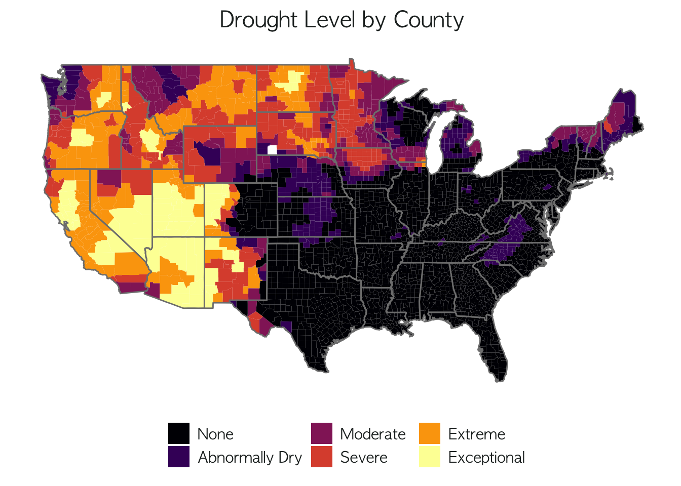
Now I can map the data. First I’m just going to do a regular map using the latest date that we have as the county fills. I’m using the viridis color palette so it looks more like a heatmap, even though the data is categorical.

 map_usa %>% 
  ungroup() %>% 
  filter(valid_start == max(valid_start)) %>% 
  ggplot(aes(long, lat, group = group)) +
  geom_polygon(aes(fill=fct_rev(drought_lvl))) +
  borders("state")+
  coord_map() +
  viridis::scale_fill_viridis(discrete = TRUE, option = "B")+
  theme_minimal()+
  labs(title = "Drought Level by County")+
  my_theme

Animate the Map

Now, I tried using transition_time from gganimate because that seemed like the most logical thing to do, but there is a lot of data and it was taking quite a long time to run. This is why I ended up using transition_manual, which I don’t think is the ideal solution. You have to have exactly 100 frames, or some factor of 100, which wouldn’t work for any dataset. You’ll notice in the tibbletime series I created, I used exactly 100 weeks.

To animate the map, all I did was add the transition. I also added a week subtitle that will change with every frame of the gif. If you’re just testing out your map styling/formatting, I would recommend filtering to the last 10 frames, as I did in the plot below (commented out). That way it runs a lot faster and you can make sure you’re happy with the look of the map before running the whole dataset.

Also commented out at the bottom of this code chunk is how I saved the gif out to a file.

p <- map_usa %>% 
  ungroup() %>% 
  #filter(valid_start > "2021-05-04") %>% 
  ggplot(aes(long, lat, group = group)) +
  geom_polygon(aes(fill=fct_rev(drought_lvl))) +
  borders("state")+
  coord_map() +
  viridis::scale_fill_viridis(discrete = TRUE, option = "B")+
  theme_minimal()+
  transition_manual(frames = valid_start)+
  labs(title = "Drought Level by County", subtitle = "Week: {current_frame}")+
  my_theme

#animate(p, renderer = gifski_renderer("drought.gif"))